On Compression, Computation and the Space Between

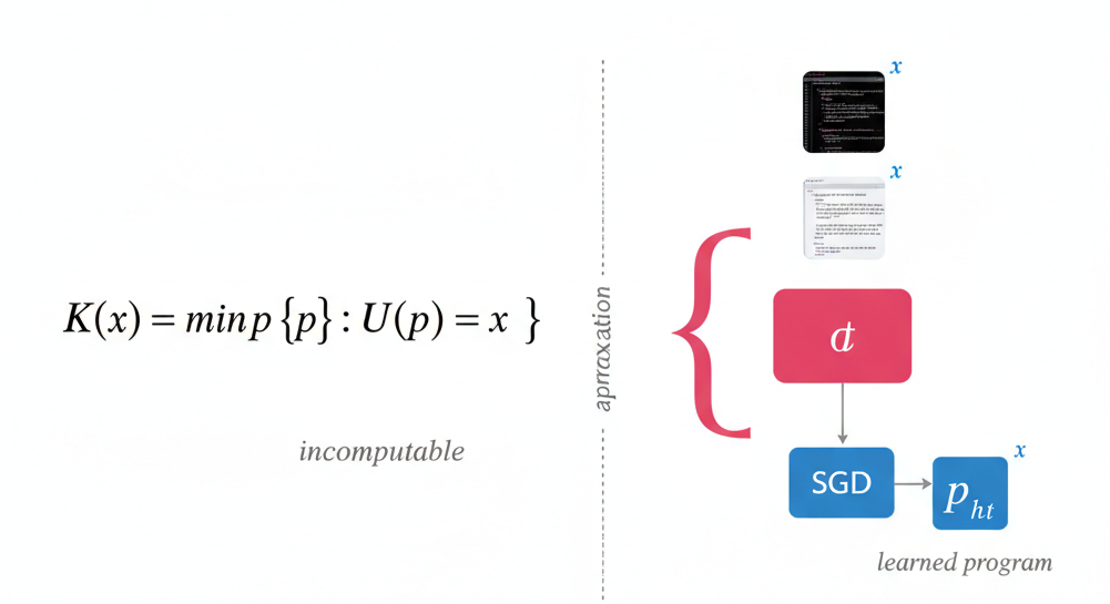
Kolmogorov and Solomonoff arrived at the same idea independently: the complexity of an object is the length of the shortest program that produces it. Fix a universal Turing machine $U$. For any finite string $x$:

$|p|$ is the length of the program in bits. This is the Kolmogorov complexity of $x$. The irreducible core. Whatever is left after you have compressed away everything you can.

The reason no scheme can beat it: if you pick a different universal machine $U'$, complexity changes by at most a constant:

$c$ depends on the machines, not on $x$. The constant is just the length of the program that lets one machine simulate the other. So if you hand me a compressor $C$ that you say is better, I write a program on $U$ that runs $C$. I pay $|C|$ extra bits. That is all. $K$ is optimal up to a constant, which for any sufficiently large dataset is negligible. $K(x)$ is not computable. Finding the shortest program means enumerating all programs and running each one, which is at least as hard as the halting problem.

There is a conditional form:

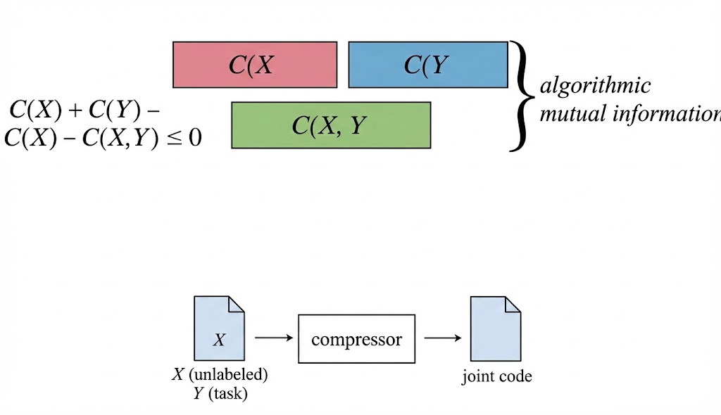
The shortest program that outputs $y$ given access to $x$. The gap $K(y) - K(y|x)$ is how much knowing $x$ helps you describe $y$. This is the algorithmic mutual information.

In a 2023 Simons Institute for the Theory of Computing talk, Sutskever laid out a framework that takes Kolmogorov complexity seriously as more than a curiosity [1]. Supervised learning has guarantees. Low training error plus fewer effective parameters than training examples gives you low test error. Three lines of math. Unsupervised learning has nothing like this. You optimize one objective (next-token prediction, denoising) but care about another (reasoning, translation). Why should the first help with the second?

Sutskever's answer: compression. Two datasets, $X$ unlabeled, $Y$ the task you care about. Compress them jointly. A good enough compressor will exploit whatever structure they share:

That gap is the shared structure. It is non-negative because compressing jointly lets the compressor reuse patterns that appear in both datasets, so it is never worse than compressing separately. The better the compressor, the more it extracts. In the limit, the Kolmogorov compressor gets all of it.

Then the step that matters. A neural network with $L$ layers is a circuit. The weights define which computation it performs. SGD adjusts the weights. So SGD is searching over the space of computations that circuit can express. The objective for autoregressive language modeling is negative log-likelihood: literally the number of bits to encode the data using the model as a codebook. Maximum likelihood is minimum description length: the negative log-likelihood of the data under a model is exactly the number of bits that model needs to encode it, so making the data more probable under the model is the same as compressing it.

Training a neural network is program search. Sutskever calls the result a "micro-Kolmogorov compressor." It cannot search all programs. SGD is not exhaustive enumeration. But scale the network, you expand what programs are expressible. The approximation to $K$ improves.

He also points out something practitioners already know in their bones: it is hard to beat existing architectures. The simulation argument explains why. If architecture $A$ can simulate $B$ cheaply, $A$ is already nearly as good as $B$ for compression. You only get a real gain when the old architecture has a bottleneck that makes simulation expensive. The RNN's fixed hidden state is one. It cannot cheaply simulate full-context attention. Give the RNN unlimited hidden state, the advantage probably vanishes.

I find this framework mostly convincing but I think it skips over the hardest part. Saying "SGD is program search" and "bigger networks approximate $K$ better" is clean in the abstract, but the actual mystery is why SGD, a local gradient method, finds good programs at all. $K$ is defined by exhaustive search. SGD is the opposite of exhaustive. The framework says what the network is converging toward. It does not say why convergence is possible. Recent work makes this tension sharper. Shaw et al. [6] constructed an asymptotically optimal description length objective for Transformers by building an explicit bridge between Transformer weights and prefix Turing machines. The theory works: a minimizer of their objective achieves optimal compression up to an additive constant as model resources grow. But they also found that standard optimizers fail to find such solutions from random initialization. The target exists. The landscape contains it. SGD cannot reach it. The gap between "the optimal program is in there" and "gradient descent will find it" is not a technicality. It is the central open problem.

Stephen Wolfram has spent decades on a different question [2]. Not compression, not learning. Just: what happens when you run simple programs? The answer, which he has verified across thousands of systems, is that most of them produce behavior far more complex than the rule that generates it. Rule 30 is the standard example. It is a one-dimensional cellular automaton: a row of cells where each cell updates based on itself and its two neighbors, with the eight-bit rule number encoding the lookup table for all possible configurations. The output passes statistical randomness tests. Deterministic. Trivial to define. Yet it produces something that looks incompressible. Wolfram's Principle of Computational Equivalence (PCE) generalizes this: past a low threshold, almost all rules are computationally universal [3]. They can all simulate each other. The differences are encoding overhead, not fundamental.

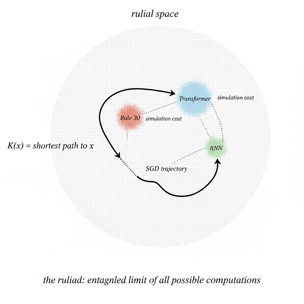
In 2021 he proposed the ruliad [4]. Run all possible rules on all possible inputs for all possible steps. Connect equivalent states across computational paths. The result is not many separate computations. It is one object: the entangled totality of everything computable, with its own topology. The ruliad is unique. Build it from Turing machines, hypergraph rewritings (rules that transform graph-like structures by replacing local patterns), string substitutions, you get the same thing. This follows from the PCE, for the same reason $K(x)$ is invariant across universal machines. Wolfram claims physics is what observers embedded in the ruliad perceive [5]. We are computationally bounded. We are temporally coherent. Those constraints determine which slice of the ruliad we see. General relativity, quantum mechanics, thermodynamics follow from observer properties, not from any particular rule.

The ruliad has geometry. Positions correspond to rules. Distance between positions is simulation cost. Nearby rules are rules that can emulate each other cheaply. It is worth noting that Wolfram's January 2026 essay "What Is Ruliology?" [7] defines the field as "the pure basic science of what simple rules do" and positions it alongside natural history: cataloguing computational creatures. Connection I am drawing here is not one he has made. Ruliology, as Wolfram practices it, is deliberately upstream of applications.

Here is what I keep thinking about. $K(x)$ is defined as a minimum over the space of all programs. The ruliad is the space of all programs, given structure. Kolmogorov treats this space as a background you optimize over. Wolfram treats it as the thing to study. They rarely engage each other but they need the same object.

The simulation argument and the PCE are, as far as I can tell, the same claim in different notation. The simulation argument: any compressor $C$ can be run by the Kolmogorov compressor at cost $|C|$ bits. The PCE: any sufficiently complex rule can simulate any other at finite cost. Past a threshold, programs are separated by translation overhead, nothing deeper. Sutskever's observation that architectures are hard to improve is the engineering face of this. But there is a real disagreement underneath the similarity. Kolmogorov complexity selects. It wants the one shortest program. The ruliad does not select. All programs run. All rules are equally present. Selection is what the observer does, not what the space does. Sutskever says the network optimizes. Wolfram says the observer samples. These are different operations. I am not sure they can be reconciled cleanly. I have not seen anyone try.

What actually interests me most is a question neither framework answers. In the ruliad, distance between rules is simulation cost. In parameter space, distance is Euclidean distance between weight vectors. These are defined on completely different substrates. There is no theorem relating them. But consider what it would mean if they were even loosely correlated in the regions that matter. If nearby points in parameter space tend to correspond to nearby points in rulial space, then the loss landscape inherits structure from the space of all computations. SGD would not be searching blindly. It would be following a surface that reflects how programs are actually organized: similar parameters, similar computations, similar compression.

There is recent evidence that the structure is real, even if nobody has named it properly yet. Valle-Pérez et al. showed in 2019 that the parameter-function map of deep networks is exponentially biased toward functions of low Kolmogorov complexity [8]. Not weakly biased. Exponentially. Simple functions occupy vastly more volume in parameter space than complex ones. Mingard et al. confirmed this in Nature Communications last year [9]: DNNs have an architectural prior toward low-$K$ functions that exactly counteracts the exponential growth in the number of functions with complexity. The bias is not learned. Even randomly initialized language models prefer to generate low-complexity sequences [10]. The architecture itself carves out a region of program space where simple programs dominate.

Mode connectivity results push this further. Good solutions found by SGD are not isolated points. They are connected by low-loss paths through parameter space [11]. Recent work has extended this from curves to surfaces [12], from parameter space to input space, from standard architectures to mixture-of-experts. The picture that emerges is not a landscape of scattered minima but a connected manifold of good programs. DeMoss et al. [13] tracked Kolmogorov complexity through training on networks that exhibit grokking — the phenomenon where a network memorizes the training data long before it suddenly generalizes. They found a characteristic pattern: complexity rises during memorization, then falls sharply when the network generalizes. The network first encodes the data as a lookup table (high $K$), then finds the short program (low $K$). Compression happens. You can watch it happen.

Then there is the SGD versus Adam result. SGD has a stronger simplicity bias than Adam. SGD finds linear decision boundaries. Adam finds richer, nonlinear ones closer to Bayes optimal — the best possible boundary given the true data distribution. This means the choice of optimizer changes where in program space you end up. Different search procedures explore different regions. The space has enough structure that how you walk through it determines what you find. None of this proves a connection to rulial geometry. But it is consistent with a picture where neural network parameterizations are smooth coordinate charts on local regions of something like the ruliad. Where simple programs form large, connected basins. Where SGD works not because it is clever but because the territory it covers is organized in its favor.

Wolfram showed simple rules make complex behavior. Kolmogorov showed complexity is measured by the simplest rule that reproduces it. Neural networks find simple rules from complex data, using a local search method that should not work but does. The missing piece is the geometry. Why the search works. What makes the space navigable. If the ruliad has the structure Wolfram says it does, that structure might be the answer. But right now this is a question. The three rooms share a wall. Nobody has opened a door.

References

[1] I. Sutskever, "An Observation on Generalization," talk at Simons Institute for the Theory of Computing, UC Berkeley, August 2023.

[2] S. Wolfram, A New Kind of Science, Wolfram Media, 2002.

[3] S. Wolfram, "The Principle of Computational Equivalence," Chapter 12 of A New Kind of Science, 2002.

[4] S. Wolfram, "The Concept of the Ruliad," Stephen Wolfram Writings, November 2021. https://writings.stephenwolfram.com/2021/11/the-concept-of-the-ruliad/

[5] D. Rickles, H. Elshatlawy, X. D. Arsiwalla, "Ruliology: Linking Computation, Observers and Physical Law," arXiv:2308.16068, 2023.

[6] P. Shaw, J. Cohan, J. Eisenstein, K. Toutanova, "Bridging Kolmogorov Complexity and Deep Learning: Asymptotically Optimal Description Length Objectives for Transformers," arXiv:2509.22445, 2025.

[7] S. Wolfram, "What Is Ruliology?", Stephen Wolfram Writings, January 2026. https://writings.stephenwolfram.com/2026/01/what-is-ruliology/

[8] G. Valle-Pérez, C. Q. Camargo, A. A. Louis, "Deep Learning Generalizes Because the Parameter-Function Map is Biased Towards Simple Functions," ICLR 2019. arXiv:1805.08522.

[9] C. Mingard, H. Rees, G. Valle-Pérez, A. A. Louis, "Deep Neural Networks Have an Inbuilt Occam's Razor," Nature Communications, 16, 220, January 2025.

[10] M. Goldblum, M. Finzi, K. Rowan, A. G. Wilson, "The No Free Lunch Theorem, Kolmogorov Complexity, and the Role of Inductive Biases in Machine Learning," ICML 2024. arXiv:2304.05366.

[11] T. Garipov et al., "Loss Surfaces, Mode Connectivity, and Fast Ensembling of DNNs," NeurIPS, 2018.

[12] J. Ren, P.-Y. Chen, R. Wang, "Revisiting Mode Connectivity in Neural Networks with Bézier Surface," ICLR 2025.

[13] B. DeMoss et al., "The Complexity Dynamics of Grokking," Physica D, 2025.

[14] B. Vasudeva, J. W. Lee, V. Sharan, M. Soltanolkotabi, "The Rich and the Simple: On the Implicit Bias of Adam and SGD," arXiv:2505.24022, 2025.